JavaScript Guide

The baselode npm package provides data loading, desurveying, 2D strip-log visualisation, and a 3D scene renderer for drillhole and spatial datasets.

Requires: Node.js 18+ · peer dependencies: React 18+, Three.js, Plotly, PapaParse

npm install baselode

---

Peer Dependencies

baselode relies on the following peer dependencies, which must be installed in your application:

npm install react react-dom three three-viewport-gizmo plotly.js-dist-min papaparse

---

Data Model

The JavaScript package exposes the same Baselode Open Data Model constants as the Python package.

import {
  HOLE_ID, LATITUDE, LONGITUDE, ELEVATION,
  AZIMUTH, DIP, FROM, TO, MID, DEPTH,
  EASTING, NORTHING, CRS,
  BASELODE_DATA_MODEL_DRILL_COLLAR,
  BASELODE_DATA_MODEL_DRILL_SURVEY,
  BASELODE_DATA_MODEL_DRILL_ASSAY,
  DEFAULT_COLUMN_MAP
} from 'baselode';

Column standardization

Like the Python loaders, the JS column utilities normalise source field names to the Baselode data model.

import { standardizeColumns, normalizeFieldName } from 'baselode';

const normalised = standardizeColumns(rawRows);
// e.g. "HoleId" → "hole_id", "RL" → "elevation"

---

Data Loading

Collars, surveys, and assays

import { loadCollars, loadSurveys, loadAssays, assembleDataset } from 'baselode';

// Accepts a CSV text string or an array of row objects
const collars  = loadCollars(collarsText);
const surveys  = loadSurveys(surveysText);
const assays   = loadAssays(assaysText);

const dataset = assembleDataset({ collars, surveys, assays });

Assay-focused loaders

For large assay CSVs with multiple analyte columns:

import { loadAssayFile, loadAssayHole, buildAssayState } from 'baselode';

// Load metadata (hole IDs + column names) without parsing all rows
const meta = await loadAssayMetadata(csvText);

// Load assay data for a specific hole
const holeData = loadAssayHole(csvText, 'HOLE_001');

Structural data

import { parseStructuralPointsCSV, parseStructuralCSV } from 'baselode';

const structuralPoints = parseStructuralPointsCSV(csvText);
// Returns an array of { hole_id, depth, dip, azimuth, alpha, beta, comments }

Block model

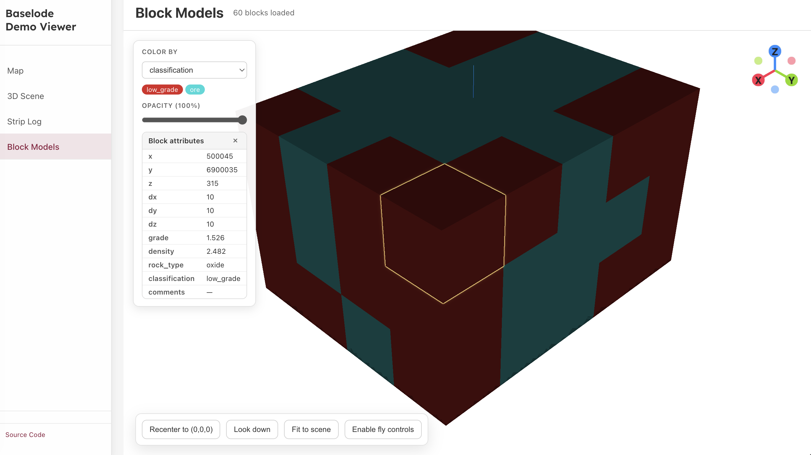
import { parseBlockModelCSV, getBlockStats, filterBlocks } from 'baselode';

const blocks = parseBlockModelCSV(csvText);
const stats  = getBlockStats(blocks, 'au_ppm');
const subset = filterBlocks(blocks, { property: 'au_ppm', min: 1.0 });

Polygonal grade blocks

Grade blocks are closed polyhedral meshes — grade shells, geologic domains, or any volumetric solid defined by triangulated vertices. They are loaded from a structured JSON format:

import { loadGradeBlocksFromJson, addGradeBlocksToScene } from 'baselode';

// Parse and validate the JSON (accepts a parsed object or a JSON string)
const blockSet = loadGradeBlocksFromJson(json);

// Render into an existing THREE.Scene (e.g. from Baselode3DScene)
const group = addGradeBlocksToScene(scene.scene, blockSet);
// Returns a THREE.Group whose children are one THREE.Mesh per block

JSON schema (version "1.0")

{
  "schema_version": "1.0",
  "units": "m",
  "blocks": [
    {
      "id": "HG",
      "name": "High grade",
      "vertices": [[0,0,0], [10,0,0], [10,10,0], [0,10,0],
                   [0,0,5], [10,0,5], [10,10,5], [0,10,5]],
      "triangles": [[0,1,2],[0,2,3], [4,5,6],[4,6,7],
                    [0,1,5],[0,5,4], [1,2,6],[1,6,5],
                    [2,3,7],[2,7,6], [3,0,4],[3,4,7]],
      "attributes": { "grade_class": "HG", "au_ppm": 4.2 },
      "material": { "color": "#B02020", "opacity": 1.0 }
    }
  ]
}

Field	Required	Description
schema_version	yes	Must be "1.0"
units	no	Coordinate units string (e.g. "m")
blocks[].id	yes	Unique identifier
blocks[].name	yes	Display name
blocks[].vertices	yes	[[x,y,z], ...] array of 3-D vertex positions
blocks[].triangles	yes	[[i,j,k], ...] zero-based triangle index triples
blocks[].attributes	no	Arbitrary key-value metadata shown in selection panel
blocks[].material.color	no	CSS hex colour (default #888888)
blocks[].material.opacity	no	0–1 opacity (default 1.0)

Unified dataset (assays + structural)

import { parseUnifiedDataset } from 'baselode';

const unified = parseUnifiedDataset(assaysCsvText, structuralCsvText);
// Returns a combined array with a `_source` tag ('assay' | 'structural')

---

Desurveying

parseSurveyCSV and desurveyTraces

import { parseSurveyCSV, desurveyTraces } from 'baselode';

const surveyTable = parseSurveyCSV(surveyCsvText);
const traces      = desurveyTraces(collarsCsvText, surveyTable);
// traces: Map<holeId, TracePoint[]> where each point has { x, y, z, md, azimuth, dip }

Low-level desurvey methods

import {
  minimumCurvatureDesurvey,
  tangentialDesurvey,
  balancedTangentialDesurvey,
  buildTraces
} from 'baselode';

// minimumCurvatureDesurvey is the industry standard (default)
const trace = minimumCurvatureDesurvey(collar, surveyRows, { step: 1.0 });

Attaching assay positions to 3D traces

import { attachAssayPositions } from 'baselode';

const assaysWithXYZ = attachAssayPositions(assayRows, traces);
// Adds { x, y, z } to each assay row by interpolating the trace

Interpolating the trace at arbitrary depths

import { interpolateTrajectory } from 'baselode';

const positions = interpolateTrajectory(traces, { 'DH001': [47.3, 52.1] });
// → [
//   { hole_id: 'DH001', depth: 47.3, x, y, z, azimuth, dip },
//   { hole_id: 'DH001', depth: 52.1, x, y, z, azimuth, dip },
// ]

Linear interpolation per coordinate. Mirrors the Python interpolate_trajectory. depths accepts a number, number[], {hole_id: [...]}, or [{hole_id, depth}, ...]. Out-of-range depths (and unknown holes) return rows with null in every output field except hole_id and depth.

---

DrillholeSet — the composition root

DrillholeSet bundles collar + survey + N named interval tables into one object, mirroring the Python class. Methods delegate to the existing function-based API.

import { DrillholeSet } from 'baselode';

const db = new DrillholeSet(collarRows, surveyRows, {
  crs: 'EPSG:32750',
  project: 'goldfields-2026',
});

db.addTable('assay', assayRows)
  .addTable('geology', lithoRows, 'litho');

const report = db.validate();
const traces = db.desurvey({ method: 'minimum_curvature', step: 1 });

OMF export (db.to_omf in Python) is intentionally Python-only; the JS class focuses on the in-memory validate/desurvey path.

---

Database validation

validateDrillholeDb mirrors the Python validator, returning a structured { summary, issues } report covering every check in one pass.

import {
  validateDrillholeDb,
  fixSingleStationSurveys,
  normalizeAzimuth,
  dropOrphanIntervals,
  swapInvertedIntervals,
  replaceBelowDetectionLimit,
} from 'baselode';

const report = validateDrillholeDb({
  collar: collarRows,
  survey: surveyRows,
  intervalTables: { assay: assayRows, geology: lithoRows },
});

const errors = report.issues.filter((issue) => issue.severity === 'error');

Checks covered (severity, what triggers): duplicate_hole_ids (error), single_station_surveys (warning), azimuth_range / dip_range (error), orphan_intervals (error), negative_lengths (error), intervals_beyond_max_depth (warning), interval_gaps (info), interval_overlaps (warning), below_detection_limit (info).

Fix helpers

const surveyFixed    = fixSingleStationSurveys(surveyRows, collarRows);
const surveyWrapped  = normalizeAzimuth(surveyRows);  // 360 → 0, -30 → 330, idempotent
const assaysMatched  = dropOrphanIntervals(assayRows, collarRows);
const assaysSwapped  = swapInvertedIntervals(assayRows);  // fixes to<from typos
const assaysClean    = replaceBelowDetectionLimit(assayRows, { columns: ['au_ppm'] });

All helpers return new arrays — the source rows are untouched.

To treat azimuth = 360 as valid without normalizing first, pass allowFullCircle: true:

const report = validateDrillholeDb({ collar, survey }, { allowFullCircle: true });

---

Interval algebra

Pure from-to primitives that mirror the Python baselode.drill.intervals module. Each function takes an array of row objects keyed by hole_id, from, to — the same shape your loaders already produce.

import {
  intervalLength,
  fromToMidpoints,
  detectGaps,
  detectOverlaps,
  splitAt,
  clip,
  mergeTables,
} from 'baselode';

QC checks: gaps and overlaps

const gaps     = detectGaps(assayRows, { minGap: 0.5 });
const overlaps = detectOverlaps(assayRows);
// gaps:     [{ hole_id, from, to, length }, ...]
// overlaps: [{ hole_id, from, to, length, first_index, second_index }, ...]

first_index / second_index are positional indices into the input array.

Splitting at boundaries

// per-hole boundaries
const splitByHole = splitAt(assayRows, { DH001: [12.5, 47.0] });

// or as a row array (handy when the boundaries come straight from a CSV)
const splitByRows = splitAt(assayRows, [
  { hole_id: 'DH001', depth: 12.5 },
  { hole_id: 'DH001', depth: 47.0 },
]);

// or broadcast a single list to every hole
const splitAll = splitAt(assayRows, [50, 100]);

Each straddling row is replaced by sub-intervals that inherit all other fields.

Clipping to a depth window

const top200m = clip(assayRows, 0, 200);

Intervals entirely outside [fromDepth, toDepth] are dropped; straddling intervals are pulled to the boundary. Pass null for either bound to disable that side.

Merging interval tables onto a common support

const merged = mergeTables({ assay: assayRows, litho: lithoRows });
// each row: { hole_id, from, to, assay_<col>, ..., litho_<col>, ... }

The first table in the object is the "left" — only depth ranges it covers appear in the output. Each subsequent table's columns are looked up at the sub-interval midpoint and prefixed by table name (or null when no covering row exists).

Per-row helpers

const lengths = intervalLength(assayRows);    // number[]
const mids    = fromToMidpoints(assayRows);   // number[]

---

3D Interpolation Volumes

baselode ships a small GPU-rendered IDW (inverse-distance-weighted) interpolation volume — the kind of "fuzzy 3D heatmap" you want for a quick look at how a drilling attribute (Au grade, alteration index, anything numeric) varies between sample points before committing to a full block model.

The stack composes four primitives so each piece is reusable on its own:

Piece	What it does
buildInterpSamplesFromAssays(rows, attribute)	Convert assay-interval rows (with desurveyed x/y/z or collar-vertical fallback) into { id, x, y, z, value } sample points
computeVolumeBounds(points, padding)	Auto-compute an axis-aligned bbox from a sample set, with optional uniform world-unit padding
IDWSampler(samples, opts)	Pure scalar-field sampler: getValueAt(x, y, z) returns the IDW-interpolated value. Backed by SpatialHash3D for fast radius queries
buildVoxelGrid(sampler, bounds, dims)	Walk the sampler across a regular voxel grid; returns { values: Float32Array, nodataMask: Uint8Array, dims, voxelSize, bounds }
IDWVolumeRenderer	Three.js shader-based volume renderer; uploads the voxel grid as a Data3DTexture and ray-marches it inside a bounding box
IDWVolumeLayer	One-call wrapper that does all of the above and exposes a Three.Object3D for the scene

Single-call workflow

import {
  IDWVolumeLayer,
  buildInterpSamplesFromAssays,
} from 'baselode';

const samples = buildInterpSamplesFromAssays(assayRowsWithPositions, 'au_ppm');

const layer = new IDWVolumeLayer({
  samples,
  idw:        { power: 2, searchRadius: 60, maxNeighbors: 8 },
  grid:       { dims: [64, 64, 64] },   // or { voxelSize: [10, 10, 10] }
  displayMin: 0,
  displayMax: 5,
  opacity:    0.6,
  threshold:  0.15,   // normalised [0,1] cutoff; null disables
  blockMode:  true,   // crisp voxel-blocks vs smooth trilinear blend
});

await layer.rebuild();
scene.add(layer.object3D);

// Display-only knobs — no rebuild required
layer.setOpacity(0.4);
layer.setThreshold(0.3);
layer.setBlockMode(false);

// Axis-aligned slice planes (per-axis bounds in [0,1] box-local space)
layer.setClipBounds([0, 0, 0], [1, 1, 0.6]);  // slice off the top 40% of Z

// Cleanup
scene.remove(layer.object3D);
layer.dispose();

How the rendering works

IDWVolumeRenderer ray-marches a Three.js box mesh in a custom GLSL 3 fragment shader. Each ray:

• Intersects the AABB clipped to the current [uClipMin, uClipMax] sub-box.
• Steps through the volume (default 64–96 samples per ray).
• Samples a Data3DTexture at each step. blockMode=true snaps to voxel centres for the crisp block-model look; false lets the GPU's trilinear filter smooth between voxels.
• Composites front-to-back with the active transfer function (blue→red by default; override via colorLow / colorHigh).
• Writes gl_FragDepth at the first significant ray hit, so opaque objects placed inside the volume (sample-point markers, drillhole traces, etc.) get correctly occluded when they sit behind the visible voxel surface and stay visible when they sit in front.

Performance guidance

buildVoxelGrid runs an async build that yields to the event loop every 4096 voxels by default — UIs stay responsive while a grid evaluates. Pass { sync: true } from inside a Web Worker.

Memory cost (Float32 values + Uint8 no-data mask):

Grid	Bytes	Notes
32³	~165 KB	Quick preview
64³	~1.3 MB	Comfortable for routine viewing
128³	~10 MB	Good for hi-detail; rebuild is noticeable
256³	~85 MB	Use with care

Cancellation tokens are honoured ({ cancellationToken: { cancelled: false } }) so an in-flight rebuild can be aborted when the user nudges a parameter.

Comparison to a full block-model estimator

This is a visualisation primitive, not a resource estimator. Use it when you want to look at the field; reach for kriging / pyGSLIB when you need to report it.

	IDWVolumeLayer	BlockModel
Run on the fly	✓	✗ (pre-computed CSV)
Tweakable interactively (power / radius / threshold)	✓	✗
Anisotropic / geological-domain aware	✗	✓
Estimator validation / variography	✗	✓ (via external tools)
Memory footprint	<100 MB	scales with rows

---

Compositing

compositeIntervals mirrors the Python composite_intervals soft + hard boundary modes. True-thickness compositing is Python-only because it needs a desurveyed trace; for browser-side workflows that need true-thickness, do the composite step server-side and ship the result to the client.

import { compositeIntervals } from 'baselode';

// Soft mode (default): fixed-length bins across each hole, length-weighted average
const composites = compositeIntervals(assayRows, 'au_ppm', { length: 2 });

// Hard-boundary by domain — composites reset at every change in the boundary column
const byLitho = compositeIntervals(assayRows, 'au_ppm', {
  length: 2,
  mode: 'hard',
  boundaryCol: 'lithology',
  residual: 'distribute',  // or 'discard' (default) / 'add_to_previous'
});

Options:

Option	Type	Default	Meaning
length	number	1	Composite length (must be a positive finite number)
method	'average' | 'sum'	'average'	Length-weighted average or sum
mode	'soft' | 'hard'	'soft'	Boundary handling
boundaryCol	string	—	Domain column for hard mode (required when mode === 'hard')
residual	'discard' | 'add_to_previous' | 'distribute'	'discard'	Tail-of-domain handling for hard mode
fromCol / toCol / holeCol	string	'from' / 'to' / 'hole_id'	Column-name overrides

Both length and method are validated up front — passing 0, NaN or Infinity for length, or an unknown method, throws with a clear message.

---

Visualization

Column classification

baselode classifies columns automatically for the strip-log renderer:

import { classifyColumns, DISPLAY_NUMERIC, DISPLAY_CATEGORICAL, DISPLAY_COMMENT, DISPLAY_TADPOLE } from 'baselode';

const classification = classifyColumns(rows);
// Returns { colName: DISPLAY_NUMERIC | DISPLAY_CATEGORICAL | DISPLAY_COMMENT | DISPLAY_TADPOLE | DISPLAY_HIDDEN }

2D strip log (Plotly)

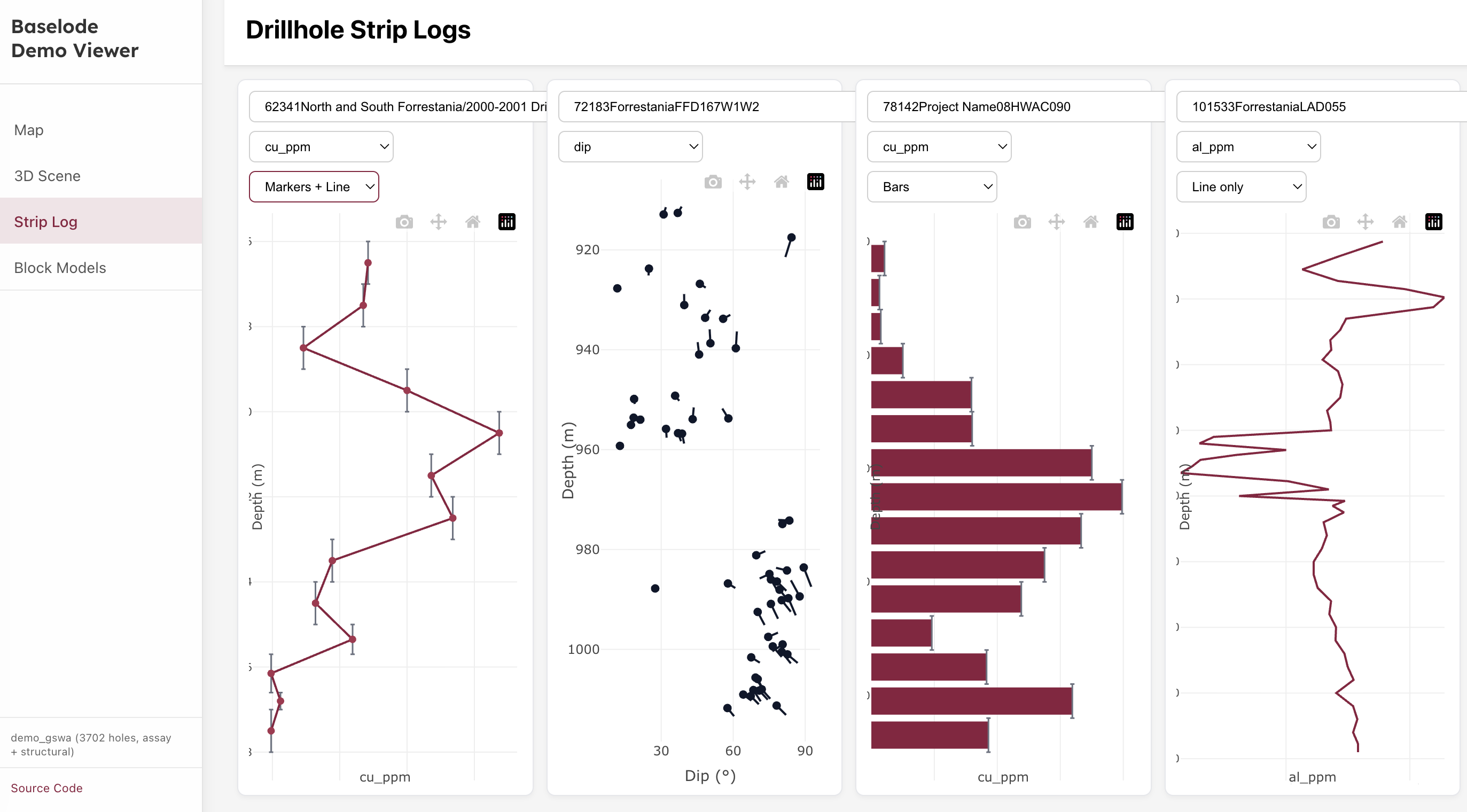
import { buildIntervalPoints, buildPlotConfig, getChartOptions, defaultChartType } from 'baselode';

const points     = buildIntervalPoints(holeRows, 'au_ppm');
const chartType  = defaultChartType('au_ppm', holeRows);
const config     = buildPlotConfig(points, 'au_ppm', { chartType });

Plotly.newPlot('container', config.data, config.layout);

React component — TracePlot

TracePlot renders a complete multi-track Plotly strip log for a single hole.

import { TracePlot } from 'baselode';

<TracePlot
  rows={holeRows}
  properties={['au_ppm', 'lithology', 'alpha']}
/>

TracePlot also accepts an optional propertyMeta map ({ [property]: { label?, unit?, sourceAttribute? } }). When the selected property has an entry, its unit / source attribute are folded into the axis title, hover tooltip and property dropdown — e.g. a column keyed Au renders as Au (ppm) — while selection and onConfigChange keep using the bare property key.

React hook — useDrillholeTraceGrid

For building full drill-hole comparison grids:

import { useDrillholeTraceGrid } from 'baselode';

function MyGrid({ holes, selectedProperty }) {
  const { plots } = useDrillholeTraceGrid({ holes, property: selectedProperty });
  return <div className="grid">{plots.map(p => <TracePlot key={p.holeId} {...p} />)}</div>;
}

Tool UI

Baselode includes a JavaScript-only Tool UI entrypoint for rendering Baselode visualisations as structured tool results.

Install zod alongside Baselode when importing baselode/tool-ui; it is a required peer dependency for the Tool UI schemas and is not bundled.

npm install baselode zod

The integration follows Tool UI's schema-first rendering pattern:

1. A backend AI SDK tool returns a structured Baselode visualisation JSON payload.
2. A Zod schema validates the result in the frontend renderer.
3. The renderer uses Baselode's existing Plotly strip-log and Three.js scene helpers inside the assistant conversation.

import { AssistantRuntimeProvider } from '@assistant-ui/react';
import { AssistantChatTransport, useChatRuntime } from '@assistant-ui/react-ai-sdk';
import { useBaselodeToolUi } from './toolkit.jsx';
import 'baselode/tool-ui/style.css';

export default function App() {
  const runtime = useChatRuntime({
    transport: new AssistantChatTransport({ api: '/api/chat' }),
  });
  const aui = useBaselodeToolUi();

  return (
    <AssistantRuntimeProvider runtime={runtime} aui={aui}>
      {/* assistant-ui thread */}
    </AssistantRuntimeProvider>
  );
}

The serializable result is intentionally compact:

{
  id: 'strip-log-BLDD001',
  hole: {
    id: 'BLDD001',
    points: [
      { from: 0, to: 12, au_ppm: 0.11, lithology: 'SAP' },
      { from: 12, to: 24, au_ppm: 0.35, lithology: 'BAS' },
    ],
  },
  tracks: [
    { property: 'au_ppm', label: 'Au ppm', displayType: 'numeric' },
    { property: 'lithology', label: 'Lithology', displayType: 'categorical' },
  ],
}

Per-property unit metadata

BaselodeStripLogToolUI accepts an optional propertyMeta map that attaches a value unit and raw source attribute to each property. The formatted label (Au (ppm), or Au (ppm, source: Au_ppb) when the source attribute differs from the display label — i.e. meta.label if provided, otherwise the bare property key) is then applied to the property selector, the track header, the axis title and the hover tooltip — selection identity and track.property still use the bare property key.

<BaselodeStripLogToolUI
  // ...
  propertyOptions={['Au', 'Cu', 'Ni']}
  propertyMeta={{
    Au: { unit: 'ppm', sourceAttribute: 'Au_ppb' },
    Cu: { unit: 'ppm', sourceAttribute: 'Cu_ppm' },
    Ni: { unit: '%' },
  }}
/>

Each entry is { label?, unit?, sourceAttribute? }. The source attribute is omitted from the display when it matches the label. propertyMeta is optional and may be partial — missing keys fall back to the bare property name.

Pass deriveMetaFromRows to back-fill metadata for keys absent from propertyMeta directly from the rows' analysis_uom / analyte_attribute columns (a unanimous value across a property's rows is adopted; a mixed set is ignored). With neither prop supplied, output is identical to the pre-metadata behaviour.

The baselode/tool-ui entry exports:

import {
  BaselodeStripLogToolUI,
  Baselode3DSceneToolUI,
  SerializableBaselodeStripLogSchema,
  SerializableBaselode3DSceneSchema,
  safeParseSerializableBaselodeStripLog,
  safeParseSerializableBaselode3DScene,
} from 'baselode/tool-ui';

Theming Tool UI chrome

Plotly-rendered strip logs use the selected Baselode Plotly template. The surrounding Tool UI chrome, including headers, controls, legends, error states, and 3D scene frames, uses CSS custom properties derived from the same Baselode light and dark palettes.

BaselodeStripLogToolUI uses light chrome by default and switches to dark chrome when template="baselode-dark". Baselode3DSceneToolUI uses light chrome by default and switches to dark chrome when background="black".

Override the CSS variables on a parent container when your app needs to theme Tool UI elements that Plotly templates do not cover:

.my-assistant-theme .baselode-tool-strip-log,
.my-assistant-theme .baselode-tool-3d-scene {
  --baselode-tool-bg: #ffffff;
  --baselode-tool-panel: #f8fafc;
  --baselode-tool-ink: #1e293b;
  --baselode-tool-ink-soft: #64748b;
  --baselode-tool-grid: #e8e8e8;
  --baselode-tool-line: #d0d0d0;
  --baselode-tool-accent: #f59e0b;
  --baselode-tool-muted-1: #94a3b8;
  --baselode-tool-muted-2: #cbd5e1;
  --baselode-tool-muted-3: #e2e8f0;
  --baselode-tool-primary: #8b1e3f;
}

Plotly templates

Baselode ships two built-in Plotly templates that can be applied to any strip log.

Export	Appearance
BASELODE_TEMPLATE / BASELODE_LIGHT_TEMPLATE	White background, Inter font, neutral grey grid
BASELODE_DARK_TEMPLATE	Dark background (#1b1b1f), Inter font, subtle warm grid

Pass a template to the low-level builder or to TracePlot:

import { buildPlotConfig, BASELODE_DARK_TEMPLATE } from 'baselode';

const config = buildPlotConfig({
  points,
  isCategorical: false,
  property: 'au_ppm',
  chartType: 'markers+line',
  template: BASELODE_DARK_TEMPLATE,   // omit to use the default light template
});

Plotly.newPlot('container', config.data, config.layout);

With TracePlot:

import { TracePlot, BASELODE_DARK_TEMPLATE } from 'baselode';

<TracePlot
  config={config}
  graph={graph}
  holeOptions={holeOptions}
  propertyOptions={propertyOptions}
  onConfigChange={handleChange}
  template={BASELODE_DARK_TEMPLATE}
/>

Building a custom template

A Baselode template is a plain object with a layout key (and optionally a data key for trace defaults) — the same shape as a Plotly template object. You do not need to register it anywhere; just pass it directly.

const MY_TEMPLATE = {
  layout: {
    paper_bgcolor: '#0f1117',
    plot_bgcolor:  '#0f1117',
    font: { family: 'JetBrains Mono, monospace', color: '#e2e8f0', size: 13 },
    colorway: ['#38bdf8', '#34d399', '#fb923c', '#f472b6', '#a78bfa'],
    xaxis: {
      showline: false,
      showgrid: true,
      gridcolor: '#1e293b',
      tickfont: { color: '#94a3b8' },
    },
    yaxis: {
      showline: false,
      showgrid: true,
      gridcolor: '#1e293b',
      tickfont: { color: '#94a3b8' },
    },
    hoverlabel: {
      bgcolor: '#1e293b',
      bordercolor: '#38bdf8',
      font: { color: '#e2e8f0', size: 12 },
    },
  },
};

const config = buildPlotConfig({ points, property, chartType, template: MY_TEMPLATE });

Colour mapping

Automatic commodity colours

Baselode automatically detects commodity elements in column names and applies a matching colour. A column called Au_ppm, au_ppb, or AU will all render in gold; Cu_pct will render in copper-brown.

No configuration is required — pass the column name to buildPlotConfig and detection is automatic.

Built-in semantic colour maps

For categorical strip logs (geology codes, lithology, alteration) two built-in maps are available:

Name	Contents
'commodity'	18 commodity elements (Au, Ag, Cu, Fe, Ni, …)
'lithology'	~30 common rock types (granite, basalt, shale, …)

import { buildCategoricalStripLogConfig } from 'baselode';

const config = buildCategoricalStripLogConfig(rows, {
  fromCol: 'from',
  toCol:   'to',
  categoryCol: 'geology_code',
  colourMap: 'lithology',          // use the built-in lithology map
});

You can also look up individual values:

import { getColour, LITHOLOGY_COLOURS } from 'baselode';

const colour = getColour('granite', LITHOLOGY_COLOURS);  // '#EF9A9A'

Custom colour maps

Supply any plain object mapping category strings to CSS colour values:

const ALTERATION_COLOURS = {
  'potassic':     '#e53e3e',
  'phyllic':      '#d69e2e',
  'propylitic':   '#38a169',
  'argillic':     '#3182ce',
  'silicification': '#805ad5',
};

const config = buildCategoricalStripLogConfig(rows, {
  fromCol:     'from',
  toCol:       'to',
  categoryCol: 'alteration_type',
  colourMap:   ALTERATION_COLOURS,
});

Lookup is case-insensitive, so "Potassic" and "potassic" both match. Categories absent from the map fall back to a built-in rotation palette.

Color scale

Continuous numeric color scales for 3D viewers and maps:

import { buildEqualRangeColorScale, getEqualRangeColor, ASSAY_COLOR_PALETTE_10 } from 'baselode';

const scale  = buildEqualRangeColorScale(values, ASSAY_COLOR_PALETTE_10);
const colour = getEqualRangeColor(scale, 2.5);  // '#...'

---

3D Scene

Baselode3DScene

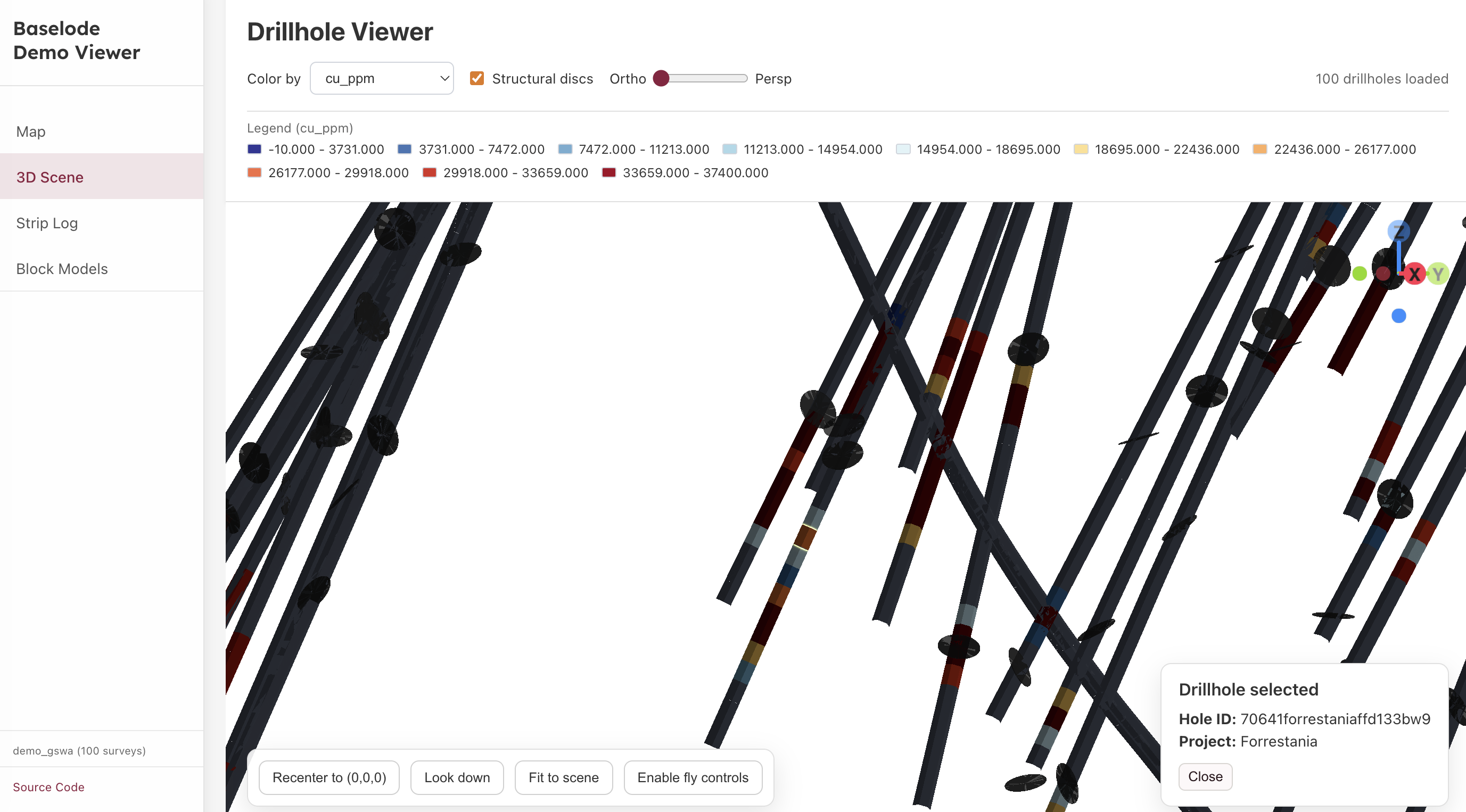
Baselode3DScene is a thin orchestrator that owns the WebGL context and delegates rendering to domain-specific modules (drillholeScene, blockModelScene, structuralScene). Use it directly or through the pre-built React wrapper.

import { Baselode3DScene } from 'baselode';

const scene = new Baselode3DScene();
scene.init(containerElement);   // attach to a DOM container

// Drillholes (desurveyed trace objects)
scene.setDrillholes(holes, { selectedAssayVariable: 'au_ppm', assayIntervalsByHole });

// Block model
scene.setBlocks(blockRows, 'au_ppm', stats);

// Structural discs
scene.setStructuralDiscs(structuralRows, holes, { radius: 5, opacity: 0.75 });

// Click handlers
scene.setDrillholeClickHandler(({ holeId }) => console.log(holeId));
scene.setBlockClickHandler((blockRow) => console.log(blockRow));

// Cleanup
scene.dispose();

React component — Baselode3DControls

Drop-in React component with orbit controls, a camera gizmo, and a controls panel:

import { Baselode3DControls } from 'baselode';
import 'baselode/style.css';

<Baselode3DControls
  traces={traces}
  structuralDiscs={discs}
  colorBy="au_ppm"
/>

React component — BlockModelWidget

Interactive 3D block model viewer:

import { BlockModelWidget } from 'baselode';
import 'baselode/style.css';

<BlockModelWidget
  blocks={blocks}
  colorProperty="grade"
/>

3D payload builders

import { tracesAsSegments, intervalsAsTubes, annotationsFromIntervals } from 'baselode';

const segments    = tracesAsSegments(traces);
const tubes       = intervalsAsTubes(assays, { colorBy: 'au_ppm', radius: 2 });
const annotations = annotationsFromIntervals(assays);

Structural disc builder

import { buildStructuralDiscs } from 'baselode';

const discs = buildStructuralDiscs(structuralPoints, traces);
// Returns Three.js-ready disc descriptors for each structural measurement

Polygonal grade blocks — 3D rendering

addGradeBlocksToScene renders each block as a THREE.Mesh with flat-shaded MeshStandardMaterial and an edge-highlight LineSegments child (hidden by default, shown on selection).

import { Baselode3DScene, loadGradeBlocksFromJson, addGradeBlocksToScene } from 'baselode';

const scene = new Baselode3DScene();
scene.init(containerElement);

const blockSet = loadGradeBlocksFromJson(json);
const group    = addGradeBlocksToScene(scene.scene, blockSet, { defaultOpacity: 0.85 });

// Register meshes so the built-in selection glow fires on click
scene.selectables = Array.from(group.children);

Click selection and edge highlight

When a mesh is clicked the scene's built-in raycast handler applies a glow outline (OutlinePass) around the outer silhouette. Each mesh also carries a hidden LineSegments child built from EdgesGeometry — showing it on selection highlights every polyhedral edge explicitly:

// Show/hide the edge overlay when selection changes
group.children.forEach((mesh) => {
  const edgeLines = mesh.children[0];
  if (edgeLines) edgeLines.visible = mesh.userData.id === selectedId;
});

mesh.userData contains { id, attributes } from the source JSON, available in the click callback.

---

Raster Overlays

A raster overlay drapes a georeferenced image (geology map, satellite photo, survey grid, etc.) as a flat plane in the 3D scene. The image is placed at a specified elevation and bounded to real-world coordinates so it aligns with drillhole traces.

Image format

Baselode3DScene uses Three.js's built-in TextureLoader, which supports formats the browser can decode natively: PNG, JPEG, WebP. GeoTIFF is not supported directly — convert it first:

# Using GDAL
gdal_translate -of PNG my_map_georeferenced.tif my_map.png

Coordinate system

Overlay bounds are expressed in the same local scene coordinate system as the drillhole traces (x = Easting offset, y = Northing offset, z = elevation in metres). If your traces are offset from a survey origin, subtract the same origin from the GeoTIFF corner coordinates:

// GeoTIFF corners in MGA zone 50 (metres):
//   Upper Left:  (693 545, 7 675 285)
//   Lower Right: (700 469, 7 667 027)
// Scene origin chosen as centroid of drillhole collars, e.g. (697 007, 7 671 156):

const ORIGIN_E = 697_007;
const ORIGIN_N = 7_671_156;

const bounds = {
  minX: 693_545 - ORIGIN_E,   // ≈ -3 462
  maxX: 700_469 - ORIGIN_E,   // ≈  3 462
  minY: 7_667_027 - ORIGIN_N, // ≈ -4 129
  maxY: 7_675_285 - ORIGIN_N, // ≈  4 129
};

Bounds can also be expressed as an origin + size object:

const bounds = { x: -3462, y: -4129, width: 6924, height: 8258 };

Loading a raster overlay

import { createRasterOverlay } from 'baselode';

const layer = await createRasterOverlay({
  id: 'geology-map',          // unique identifier (auto-generated if omitted)
  name: 'Regional geology',   // display name
  source: { type: 'url', url: '/maps/geology.png' },
  bounds,                     // placement bounds in scene coordinates
  elevation: 350,             // Z position (metres above datum); default 0
  opacity: 0.85,              // initial opacity 0–1; default 1
  visible: true,              // initial visibility; default true
});

scene.addRasterOverlay(layer);

Loading from a browser File object

When the user uploads a file via <input type="file">:

const [file] = event.target.files;
const layer = await createRasterOverlay({
  source: { type: 'file', file },
  bounds,
  elevation: 350,
});
scene.addRasterOverlay(layer);

Supplying a pre-built Three.js texture

import * as THREE from 'three';

const texture = new THREE.TextureLoader().load('/maps/geology.png');
const layer = await createRasterOverlay({
  source: { type: 'texture', texture },
  bounds,
});
scene.addRasterOverlay(layer);

Runtime controls

Opacity, visibility, and elevation can be changed at any time without recreating the overlay:

scene.setRasterOverlayOpacity('geology-map', 0.5);
scene.setRasterOverlayVisibility('geology-map', false);
scene.setRasterOverlayElevation('geology-map', 400);  // shift Z

Listing and removing overlays

// Retrieve a layer by id
const layer = scene.getRasterOverlay('geology-map');

// List all active overlays
const layers = scene.listRasterOverlays();

// Remove one overlay and free its GPU resources
scene.removeRasterOverlay('geology-map');

// Remove all overlays
scene.clearRasterOverlays();

Complete example (React)

import { useEffect, useRef } from 'react';
import { Baselode3DScene, createRasterOverlay } from 'baselode';

const BOUNDS = { minX: -3462, maxX: 3462, minY: -4129, maxY: 4129 };

export default function MapScene({ holes }) {
  const containerRef = useRef(null);
  const sceneRef = useRef(null);

  useEffect(() => {
    const scene = new Baselode3DScene();
    scene.init(containerRef.current);
    sceneRef.current = scene;

    scene.setDrillholes(holes, { preserveView: false });

    createRasterOverlay({
      id: 'geology',
      source: { type: 'url', url: '/maps/geology.png' },
      bounds: BOUNDS,
      elevation: 350,
      opacity: 0.8,
    }).then((layer) => scene.addRasterOverlay(layer));

    const onResize = () => scene.resize();
    window.addEventListener('resize', onResize);
    return () => {
      window.removeEventListener('resize', onResize);
      scene.dispose();
    };
  }, []);

  return <div ref={containerRef} style={{ width: '100%', height: '100vh' }} />;
}

---

Camera Controls

Programmatic camera control helpers for the 3D scene:

import {
  fitCameraToBounds,
  recenterCameraToOrigin,
  lookDown,
  pan, dolly,
  setFov
} from 'baselode';

fitCameraToBounds(scene, bounds);
lookDown(scene);
setFov(scene, 45);

---

Standalone Bundle

For non-React environments (e.g. embedding in a plain HTML page or a Python Dash iframe), baselode ships a standalone UMD/IIFE module that registers itself as window.baselode:

<script src="baselode-module.js"></script>
<script>
  const scene = new window.baselode.Baselode3DScene(document.getElementById('canvas'));
</script>

The standalone bundle is built from vite.standalone.js in the JS package and is copied to demo-viewer-dash/assets/ automatically:

cd javascript/packages/baselode
npm run build:module